Only a handful of macronutrient ions set the mineral side of a tissue culture medium. Finding the best mix of them is still one of the harder experiments to run well. There are too many ingredients to test by hand, they don't act independently, and the obvious way to set the experiment up muddles the answer before you start. The approach below keeps it both doable and statistically sound. You work in ions rather than salts, express everything in charge equivalents so the recipe always balances, and use an I-optimal design to cover the space in a run count a working lab can actually prepare.
Optimize ions, not salts
It's tempting to design the experiment around the salts you weigh out: KNO₃, CaCl₂, MgSO₄. The trouble is that every salt delivers two ions at once, so a "calcium nitrate effect" is really a calcium effect tangled up with a nitrate effect, and you can never cleanly separate the two. The fix, following Niedz & Evens' work on ion confounding, is to make the individual ions the experimental factors and let software back-solve which salts to weigh to hit them.
For most media that comes to four cations (ammonium NH₄⁺, potassium K⁺, calcium Ca²⁺, magnesium Mg²⁺) and three anions (nitrate NO₃⁻, phosphate, and sulfate SO₄²⁻).
Charge equivalents make electroneutrality free
We parameterize everything in charge equivalents (meq) rather than moles. The cation equivalent-fractions sum to one, the anion equivalent-fractions sum to one, and a single scalar, the total ionic charge, scales both sides. Since both sides scale to the same total, the positive and negative charges always match.
Electroneutrality holds automatically. There's no balancing step and no impossible recipes: every point in the design is electrically neutral by construction. That's what lets us treat the proportions and the overall strength as clean, independent knobs.
For this design we just count charges: the total charge equivalents on each side, with each ion weighted by its valence |z| (a Ca²⁺ counts as two). That's all the scalar is, a head-count of charge.
It is not the formal ionic strength I = ½·Σ c·z², which
weights charge squared to gauge a solution's electrostatic
non-ideality. That's a different quantity, and it diverges from our count as
soon as divalent ions (Ca²⁺, Mg²⁺, SO₄²⁻) carry a meaningful share. We call
ours total ionic charge to keep the two straight: it's a
count of charge, not a calculation of electrostatic strength.
Ionic strength measures electrostatic interaction, and an interaction always involves two charges multiplied together, so charge enters twice. A more highly charged ion creates a stronger field (it tugs on its neighbours harder) and also responds more strongly to the fields around it. Each of those scales with the charge, so the combined electrostatic impact scales with charge squared.
A divalent ion therefore contributes 4× the electrostatic effect of a monovalent, not 2×. That's the gap from a plain equivalent count, which weights by |z| because it only asks how much charge is present, not how strongly it interacts.
For the design itself, none of this needs computing. We only ever count up the charges (the |z| sum). The squared formula is here just to show what total ionic charge isn't.
The design space is smaller than it looks
Written in equivalents, the whole salt space is a product of three pieces: the cation blend, the anion blend, and the total ionic charge. Each mixture has one fewer free direction than it has components, so the real dimensionality stays modest.
The region is bounded, not the full simplex
In practice you never want the whole simplex. Many corners are biologically meaningless or impossible to make, like a medium that's all phosphate or one with no potassium at all, so each ion gets realistic limits. A typical anion set might hold NO₃ between 40% and 90% of the anion charge and PO₄ between 5% and 20%, letting SO₄ take up whatever is left. The cations get their own windows (say NH₄ 5–60%, K 10–60%, calcium and magnesium each 20–40%).
Those limits turn the clean simplex into an irregular convex region, the shaded sub-regions in Figure 1. This is where classical mixture designs (simplex-lattice, simplex-centroid) break down, because they assume the full simplex with every component free from 0 to 100%. A bounded region is an extreme-vertices problem, and an I-optimal design over the constrained polytope handles it directly. That's one more reason the optimal-design approach fits here.
The bounds also interact. You can't hit NO₃ = 90% and PO₄ = 20% at once, since they'd sum to 110% and force SO₄ negative, so that corner just gets clipped. The feasible region is the intersection of every limit. The candidate generator only ever samples inside it, and the salt LP guarantees each chosen point can actually be weighed out. So the design spends all of its runs where you'd really formulate, and the model is sharpest in the region that matters.
Mixture, mixture-amount, and mixture-process
These are distinct design families, and the distinction is about the nature of the extra variable, not how many levels it has:
- Mixture: only the proportions vary; the total is fixed.
- Mixture-amount: the proportions vary and the total amount of the blend itself varies. Varying total ionic charge is a mixture-amount factor.
- Mixture-process: the proportions vary alongside an external factor that isn't part of the blend, such as temperature, photoperiod, or pH.
Optimizing both blends plus the total charge is a mixture-mixture-amount design. pH would be the natural mixture-process axis to add later; for now we hold it fixed.
Choosing the runs: I-optimal design
We can't run every blend, so we pick a subset that estimates the model as precisely as possible. We use an I-optimal design, which minimizes the average prediction variance over the whole region. That's the right objective when the goal is to map the response surface and predict the best recipe, as opposed to D-optimal, which sharpens individual coefficients.
How many runs, and why ~39?
The run count falls out of the model rather than a guess. A full quadratic model over the six independent factors has:
| Term type | Count |
|---|---|
| Intercept | 1 |
| Linear (main effects) | 6 |
| Pure quadratic (curvature) | 6 |
| Two-factor interactions | 15 |
| Total estimable terms | 28 |
A design can't estimate 28 terms in fewer than 28 runs, and a usable design
needs a margin above that minimum for two things. A few replicated
points measure pure experimental noise independently of the model, and
a few extra lack-of-fit points test whether the quadratic
actually fits. A standard sizing is roughly 28 + 6 + 5 ≈ 39 runs,
which leaves 11 residual degrees of freedom: a healthy margin rather than a
saturated design.
Why not just run more? Without an optimal design, the conventional ways to cover this space balloon fast. A classical crossed mixture design (a simplex-centroid for the four cations at 15 blends, crossed with a simplex-centroid for the three anions at 7 blends, crossed with three charge levels) is 15 × 7 × 3 = 315 runs before any replication, and a factorial grid over the six factors is larger still. Almost all of those runs are redundant for fitting the 28-term model. They exist only to tile the region.
The thing to understand is that not every run does the same statistical job. The first 28 runs just make the model estimable: with fewer than 28, the design matrix is singular and the coefficients can't be solved at all. The next handful buy error degrees of freedom, the ability to estimate the noise and test whether an effect is real rather than merely draw a curve through the points. Past that, each extra run only shaves the prediction variance, with steep diminishing returns. A 315-run grid spends hundreds of runs far out on that flat tail. An I-optimal design instead places each run where it cuts prediction variance the most, landing you at the knee of the curve near 39 rather than out on the plateau. You don't need to visit every blend. You need enough well-placed points to pin the 28 coefficients and still estimate the error.
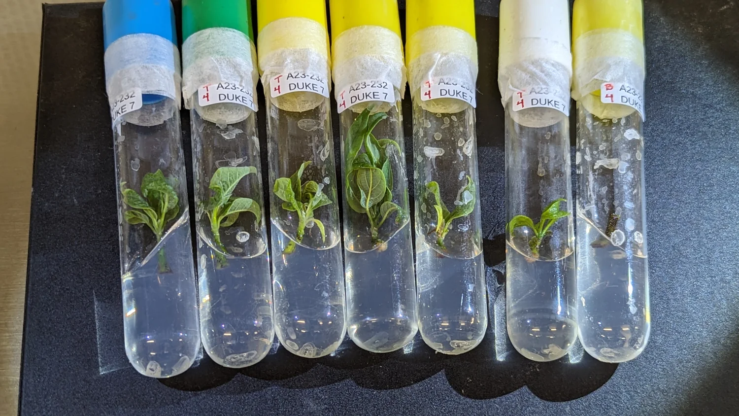
In tissue culture the scarce resource isn't plants. It's the number of distinct media you can prepare, and the design is sized to minimize that number.
Smaller questions need far fewer runs. A linear screen of the cations alone at a fixed charge is only four terms, about 14 runs. Dropping interactions or holding one blend fixed trims the model, and the run count with it.
From ions to a recipe: the salt LP
Each selected design point is a set of target ion concentrations. A small linear program back-solves the non-negative amounts of real salts that hit those targets exactly, minimizing the number of distinct species, and outputs grams per litre plus a stock-solution sheet. Points that can't be realized from the available salts are flagged as infeasible before they ever reach the bench.
Designing around the realities of the bench
A statistically clean design is only useful if it can actually be run. Three practical constraints shape ours:
- pH is held near 5.5. It pins phosphate to the monovalent H₂PO₄⁻ species (a clean −1 charge for the equivalents math), defines the calcium–phosphate solubility boundary that trims the infeasible corner of the space, and reduces precipitate at the bottom of autoclaved media.
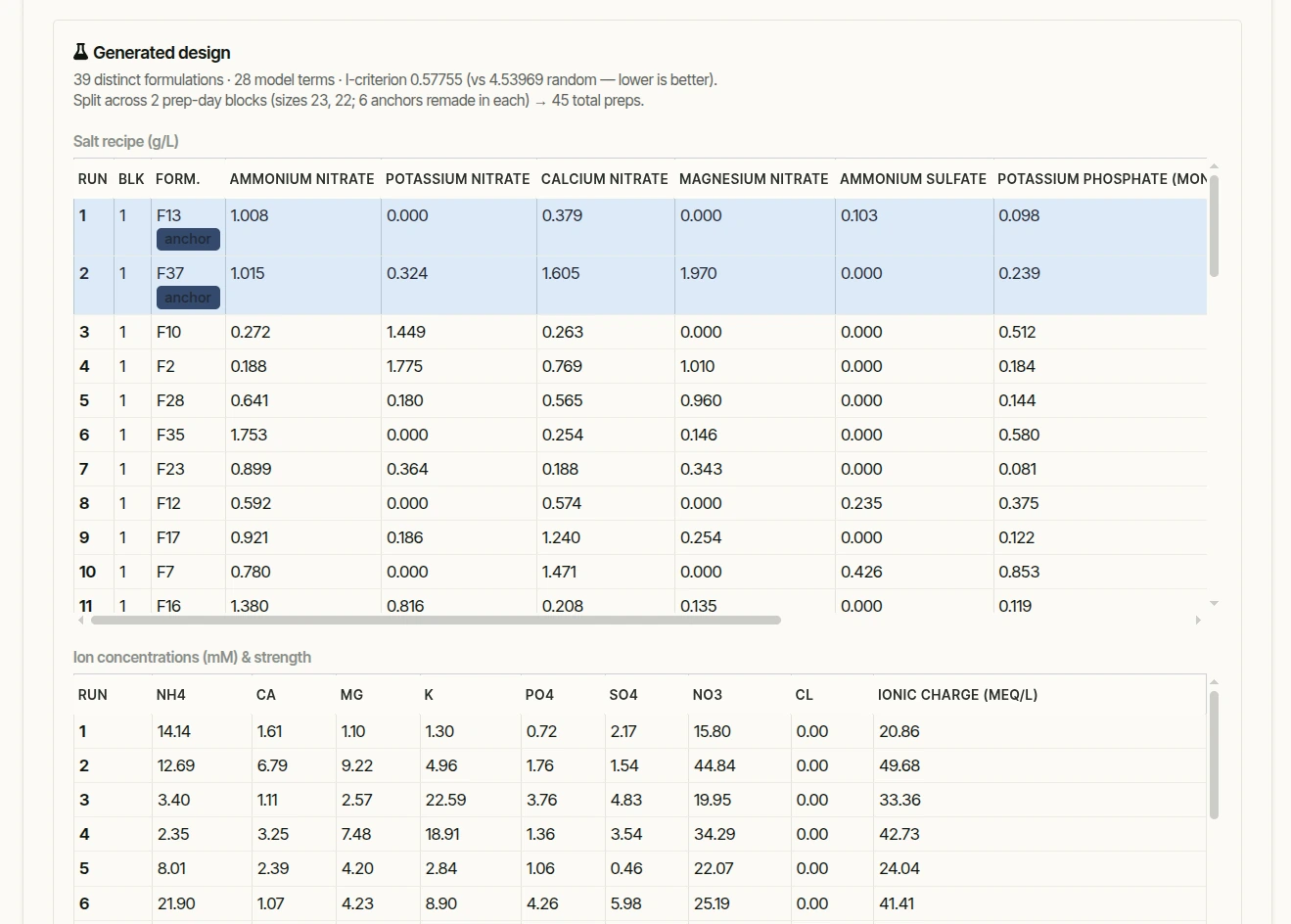
- Media prep is the real bottleneck. Each formulation is its own weigh-out, dissolve, pH-adjust, autoclave and pour, and 39 of those in a single day is a genuine stretch, not a routine afternoon. Plants, by contrast, are cheap: thousands go into the same experiment easily. The count of distinct media is the scarce resource, which is what the I-optimal design minimizes, and it's why the prep almost always spans more than one day.
- Blocking adds runs, on purpose. Once prep spans two or more days, the day (and its autoclave batch) becomes a nuisance factor, so it's treated as a block and a few anchor formulations are remade in every block to estimate and subtract that day-to-day shift. That replication is real extra work: 39 distinct media across two blocks with six anchors is about 45 actual preps, not 39. Blocking trades those few runs for protection against batch variation confounding the salt effects, a trade almost always worth making.
Reading the results
Every formulation is scored on the responses that matter (multiplication rate, shoot length or vigour, fresh weight), alongside the failure modes you want to keep down, such as contamination and hyperhydricity, tracked as their own rates. These all come off the same set of media, so measuring more responses costs more observation, not more runs.
For each response you fit the model the design was built for, the quadratic mixture / mixture-amount surface. The fit shows which ions and interactions actually move that response (a real Ca↔Mg antagonism, say, or a strong nitrate effect), and because the design carries error degrees of freedom, whether those effects are signal or noise.
A regression built for mixtures
And yes, this is not ordinary regression. The mixture constraint (the fractions sum to a fixed total) makes a standard polynomial impossible to fit, because the intercept and the component columns are perfectly collinear and the design matrix is singular. Mixture experiments use the Scheffé canonical polynomial instead, which folds the constraint into the model. Its quadratic form drops the intercept and the squared terms, keeping only the linear and cross terms:
ŷ = Σ βᵢ·xᵢ + Σ βᵢⱼ·xᵢxⱼ (i < j)
The coefficients read differently from a normal regression. Each
βᵢ is the expected response at the pure component, a vertex
of the simplex, not a slope. Each cross term βᵢⱼ measures
nonlinear blending: positive means synergy (the blend beats the
straight-line average of its two pure components), negative means antagonism. A
significant negative Ca·Mg term is the calcium–magnesium antagonism,
written as a single number.
The fitting itself is ordinary least squares; only the terms are special, and the I-optimal design was built to estimate this exact set. In practice we fit the mathematically equivalent reduced form (one component dropped, an ordinary polynomial in the remaining independent coordinates), which gives identical predictions with a well-conditioned matrix. Total ionic charge enters by crossing these mixture terms with a quadratic in charge, the mixture-amount model, so the surface can bend in both the blend and the strength.
After that it's standard regression inference. An analysis of variance over the terms flags which ions and blends are significant, the replicated runs give a lack-of-fit test (does the quadratic actually describe the data, or is it missing curvature?), and the residuals get the usual checks before any predicted optimum is trusted.
Reading it as biology, not statistics
Scheffé coefficients are precise but not intuitive. "The response at pure magnesium" isn't how a biologist thinks about a medium, so the fitted model gets translated into a few pictures that answer the questions people actually ask.
What does each ion do? A trace plot answers that directly. Starting from a reference blend, it walks each ion up (proportionally trading off the others) and draws the predicted response. One glance shows which ions are already near their best, which want more, and which are doing harm.
Which factors actually matter? An effects chart ranks the model terms by how strongly they move the response and colours them by direction, so the few real drivers (and the interactions, like a Ca·Mg antagonism) stand out from the noise.
Two more translations are worth keeping on hand. When several responses compete, a desirability map blends them into a single "goodness" surface over the mixture, so the best all-round compromise is just the brightest spot. And in the end the result is delivered as a recipe, not a model: the predicted best blend printed beside the current medium, in mM per ion and grams per litre of each salt, with the expected improvement. The experiment ends in something you can weigh out on Monday.
The real value is prediction. The fitted surface gives a predicted response at every point in the feasible region, not just the runs you made, so you can read off the blend that maximizes multiplication or minimizes hyperhydricity, including recipes you never mixed. When responses pull in different directions, a desirability function reconciles them into a single best compromise, which you then confirm with a small follow-up.
Most of that analysis is visual. The standard plot for a mixture experiment is a response surface over the blend: the predicted response drawn as a heatmap across the mixture triangle, so the optimum and the trade-offs are something you see, not just a number in a table.
Total ionic charge gets its own view. Because it enters the model as a quadratic, plotting predicted response against the charge level traces a curve with a peak (the strength the medium actually wants) inside a prediction band that widens where the data is thin.
Beyond the salt mix: where the model stops
Optimizing the salt mix is one decision among several, and the experiment assumes the others are held fixed. A few of them shape what the response surface even means.
Subculture duration, and how many passages you score. The length of a pass (two weeks, four, six) has to be chosen and then held, because the medium is a different thing at week two than at week four. Some effects, like creeping vitrification or slow salt toxicity, only surface after several consecutive passes on the same formulation, so for those you carry the lines through two or three passages rather than judging on one. Either way, duration and passage count become fixed conditions of the experiment rather than variables. Otherwise they confound the salt effects you're trying to read.
The concentration you prepared is the only one you actually know. From the moment the vessel is sealed it starts to move. The plants draw nutrients out, and, more importantly, water evaporates from the agar, so the salts that remain concentrate. A medium poured at 30 meq/L can be meaningfully stronger by the end of a four-week pass. The salt strength the plant experiences is really a trajectory, and the model fits the response to the starting point, averaged over the pass.
The salt mix interacts with the environment. Ion uptake is driven in part by transpiration, so at lower humidity, with more transpiration and more xylem flow, the plant pulls ions up quite differently than it would in a near-saturated vessel. The best blend under one humidity, light level, or vessel type is not guaranteed to be best under another.
So the response surface is an approximation, not the whole truth. It models the response to the medium as prepared, integrated over a fixed duration in a fixed environment. That's why those conditions are held constant across the experiment, why the optimum is best read as "best for this vessel, this pass length, this growth room," and why a medium worth adopting gets re-checked when any of them change. The salt mix is the part you can pin down cleanly. The rest is the context it has to live in, and being clear about that context is what keeps the result trustworthy.
Optimize ions instead of salts to avoid confounding. Work in charge equivalents so every recipe stays balanced. Pick an I-optimal subset to map the surface in the fewest distinct media, back-solve to salt weights with a linear program, and fit a response surface to each measured response to find and visualize the blend that performs best. The result is a media-optimization experiment that fits a working lab, and it points at a recipe you haven't tried yet.